基于Python scipy库实现曲线拟合
上传时间:2023-06-25
Author: Kenny Chu
主页: https://kennyangel.github.io/
Date: 20210820
一、指数函数、幂函数拟合
1、官方案例展示
使用 scipy.optimize 中的 curve_fit 函数拟合
- 定义待拟合函数方程,如 $y = func(x,a,b,c)$ ,其中 $x$ 为自变量,$a、b、c$ 为待求解系数
- 给定一组测量数据的 x 数组,如 x = [0, 10, 20, 30, 40, 50]
- 给定一组测量数据的 y 数组,如 y = [40.1, 48, 11, 88, 91, 14]
- 调用 curve_fit 函数拟合 $func$ ,如 popt, pcov = curve_fit(func, xdata, ydata)
- 捕捉函数拟合结果,popt 为一个数组,popt[0]、popt[1]、popt[2] 分别对应 $func$ 方程的三个系数 $a、b、c$
- 重新调用函数 $func$ 计算拟合后的 y 值
- 借用 matplotlib 将拟合前后的数据绘图对比
x# encoding: utf-8# version: 3.8# 案例1
from scipy.optimize import curve_fitimport matplotlib.pyplot as pltimport numpy as np
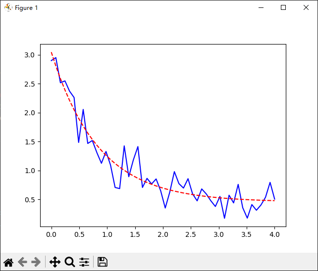
def func(x, a, b, c): return a * np.exp(-b * x) + c
xdata = np.linspace(0, 4, 50)y = func(xdata, 2.5, 1.3, 0.5)# 加入噪声ydata = y + 0.2 * np.random.normal(size=len(xdata))plt.plot(xdata, ydata, 'b-')popt, pcov = curve_fit(func, xdata, ydata)# popt数组中,三个值分别是待求参数a,b,cy2 = [func(i, popt[0], popt[1], popt[2]) for i in xdata]plt.plot(xdata, y2, 'r--')plt.show()
print(popt)上述案例计算结果如下图所示,其中红色虚线为拟合结果。
2、蠕变方程计算
使用以上方式,实现修正时间硬化蠕变方程的拟合。
修正时间硬化蠕变方程表达式如下:
修正时间硬化蠕变方程拟合源码如下:
xxxxxxxxxx# encoding: utf-8
# -----------------------------------------------------------# author  : Kenny Chu# data    : 20210820# des     : Creep - Modified time hardning. Solve C1\C2\C3\C4 by curve fitting.# version : 3.8# -----------------------------------------------------------

from scipy.optimize import curve_fitimport matplotlib.pyplot as pltimport numpy as np
# global parameter ----------------g_stress = 100  #MPag_T = 26        #℃
def f_creep_strain(t, stress, temp, c1, c2, c3, c4):    '''    基于修正时间硬化的蠕变应变方程
    :param t: 时间    :param stress: 应力状态    :param temp: 温度状态    :param c1: 系数C1    :param c2: 系数C2    :param c3: 系数C3    :param c4: 系数C4    :return: 蠕变应变方程(Modified time hardning)    '''    f = c1 * (stress**c2) * (t**c3) * (np.exp(-c4/temp))    return f
def f_creep_strain2(t, c1, c2, c3, c4):    '''    基于修正时间硬化的蠕变应变方程
    :param t: 时间    :param c1: 系数C1    :param c2: 系数C2    :param c3: 系数C3    :return: 蠕变应变方程(Modified time hardning)    '''    f = c1 * (g_stress**c2) * (t**c3) * (np.exp(-c4/g_T))    return f
# read csv --------------------------------x0 = []y0 = []
f = open('data.csv')lines = f.readlines()
for line in lines:    line = line.strip('\n')    if line != '' :        s = line.split(',')        x0.append(float(s[0]))        y0.append(float(s[1]))
print(x0)print(y0)plt.plot(x0, y0, 'b-')
# curve fitting --------------------------------
popt, pcov = curve_fit(f_creep_strain2, x0, y0)# popt数组中,四个值分别是待求参数c1,c2,c3,c4y2 = [f_creep_strain2(i, popt[0], popt[1], popt[2], popt[3]) for i in x0]plt.plot(x0, y2, 'r--')plt.show()
print(popt)
上述案例计算结果如下图所示,其中红色虚线为拟合结果。
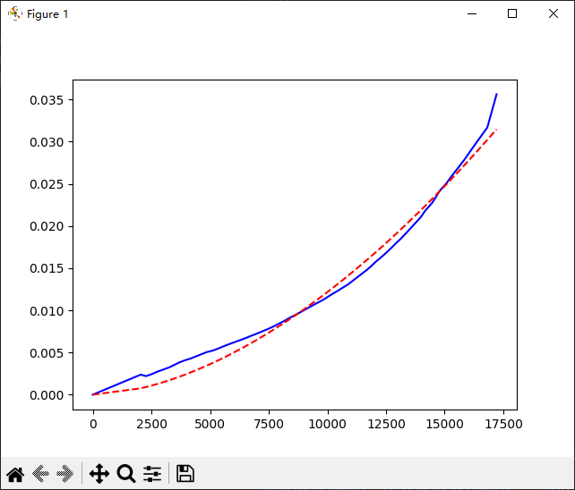
附件,"data.csv"文件内容如下。
xxxxxxxxxx0,02045.83959,0.0023777152267.589628,0.0021979332516.550037,0.0024347052762.198865,0.002738013001.073431,0.0029746313236.586049,0.0032112013465.425138,0.0035142553701.000715,0.0038340563939.887872,0.0040873224175.375307,0.0042906014861.779251,0.0050499485087.143069,0.0052031375319.293739,0.0054396575551.469593,0.0057094695786.994803,0.0059626856500.269145,0.0066891436735.806946,0.0069590056971.332156,0.0072122217206.869957,0.0074820847442.407759,0.0077519467677.970744,0.0080551018145.77254,0.0087112978374.661995,0.0090809358606.888215,0.0094173328835.752488,0.0097536789064.629352,0.0101066699293.506216,0.0104596619525.745027,0.0108127049757.971247,0.01114919986.873294,0.01153538410212.42599,0.01193826410441.31544,0.01230790210892.40823,0.01309701511259.45233,0.01388486911697.21065,0.01482359511862.24829,0.01522556812077.84105,0.01579475812296.7454,0.01629741312512.31298,0.0168333112727.90574,0.01740249912936.7872,0.01798823313088.36445,0.01837335913149.00542,0.01854072613354.53753,0.01914305613984.65718,0.02105012414173.50546,0.02181866314476.79847,0.0227720214787.14275,0.02415827615087.06122,0.02509493715238.80216,0.02569646115821.99306,0.02778593116294.07598,0.02965733916816.68886,0.03166267217213.02094,0.035613678